Anyone can create write an article here! Simply make a PR to the sherbert repo or ask us on Discord!
Changes usually take effect within ~10min of being approved.

The impasse

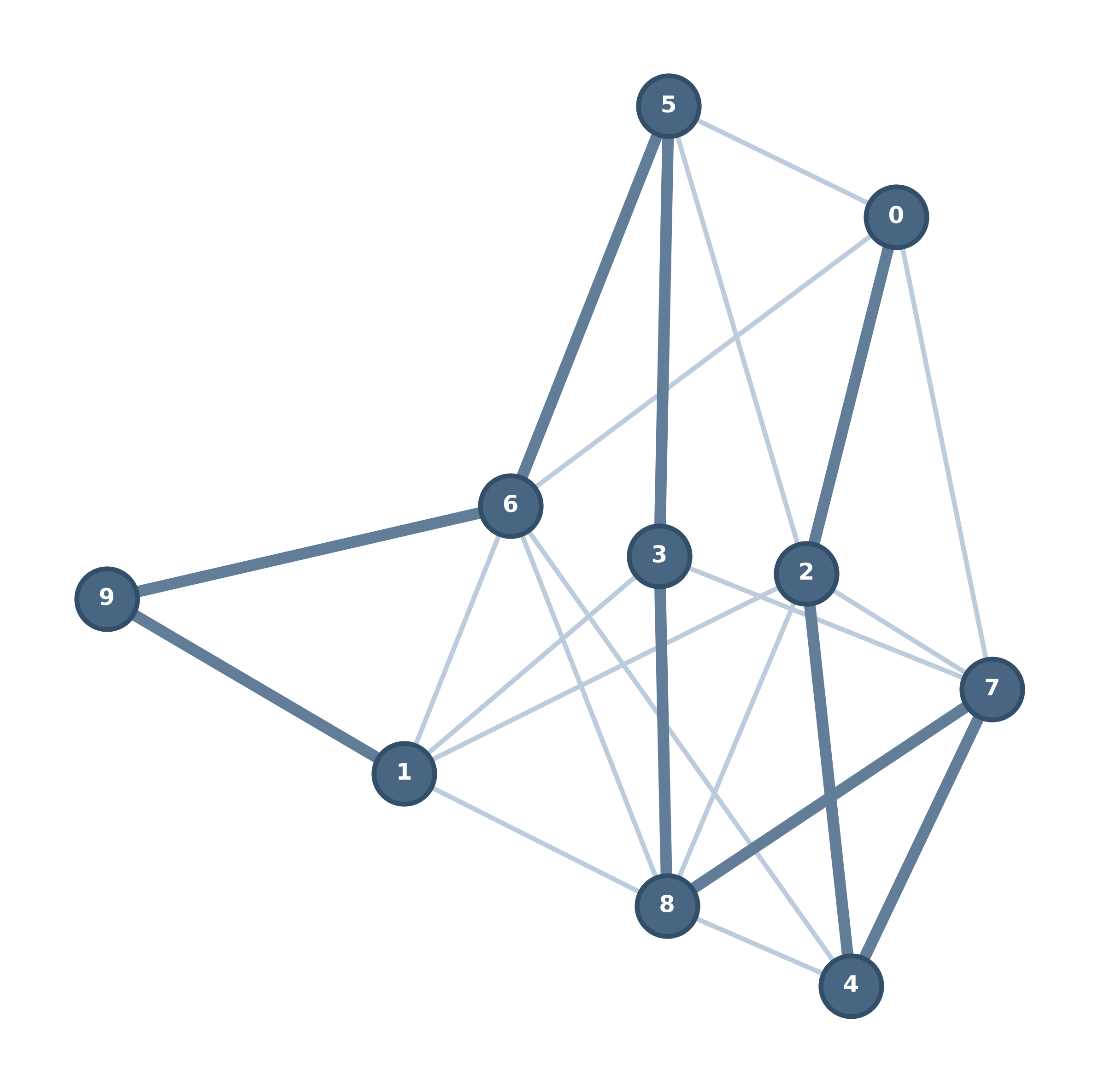
The longest path problem asks: what's a simple path of maximum edge weight between vertices in a graph? What's special about it is the lack of a known "quick" algorithm for computing the path. Here, the word "quick" means that the execution time can be expressed as a polynomial function of the input size. Also, what's a graph in this case? To be more accurate, it is:

• Undirected

• Simple

• Cyclic^[1]Which is essential! There exists an algorithm for acyclic graphs with the time complexity of O(n).

• Unweighted

There are of course methods faster than brute-force (which is $\mathcal{\text{O}}(\text{n}! \cdot \text{n})$ ). One example is the Held-Karp algorithm, where the time complexity is $\mathcal{\text{O}}(2^\text{n} \cdot \text{n}^2)$ (where $\text{n}$ means the number of nodes, as in the entire article).

That's correct, but a brute-force algorithm's space complexity depends linearly on the number of nodes, whereas Held-Karp's complexity grows as $\mathcal{\text{O}}(2^\text{n} \cdot \text{n})$ . Which means that at 30 nodes, the program would consume over 100 GB of RAM. Of course, there are certain low-level optimizations, such as capping the maximum number of nodes to 64 and using bitmasks inside a uint64_t for edge storage. While these modifications do not affect the inherent time complexity, they could reduce the constant factors.

But what about heuristics? They can be accurate or rough, fast or slow. Why not find a method to determine the near-exact longest path that finishes working within acceptable time limits? Now we bump into yet another obstacle: the longest path is notoriously hard to approximate. To put it informally, the main issue is that making optimal local choices doesn't necessarily lead us to the globally most extended path without the expensive exploration we're attempting to dodge.

The heuristic & general implementation

All aspects of the problem point to neural networks. Let's try to train a model and see how well it performs. However, we're facing a core contradiction: how to get training data if there's no way to do it within a reasonable timespan? I won't be original here: the most realistic way is to leave it searching for the longest path in the background while you're using your computer. I've done exactly this and I'm pretty sure my dataset has some entries that have taken tens of minutes to process. These are of course the best examples to feed to the network. Here's how I save a given generation:

{
  "num_nodes": 39,
  "num_edges": 72,
  "longest_path": 36,
  "adjacency_list": [
    [
      3,
      15,
      20,
      25
    ],
    [
      20,
      22,
    ...
}

This is not the only way to structure the dataset, but this one seems good enough.

The incredibly witty algorithm that searches for the longest path is written in C. Here are the constraints that I use for the last chunk of the training data:

#define MAX_NODES 64
#define MIN_DEGREE 2.5
#define MAX_DEGREE 4.1

On other runs, these constants are slightly different: we want to gather diverse entries.

One might notice that MIN_DEGREE and MAX_DEGREE are counter-intuitively used as floats. To understand why that is the case, we should dive into what these really mean. First, it stochastically calculates a value that is proportional to total edge count:

igraph_real_t target_degree = MIN_DEGREE + ((double)rand() / RAND_MAX) * (MAX_DEGREE - MIN_DEGREE)

Then, if $\text{p}$ is the probability that two given nodes become linked and $\text{d}$ is target_degree,
$\text{p} = \begin{cases} 0, & \text{if } \text{n} \in \{0, 1\} \\ \text{min}\left(1.0, \frac{\text{d}}{\text{n} - 1}\right), & \text{if } \text{n} > 1 \end{cases}$

And it puts edges between every pair of nodes using $\text{p}$ .

Like this, I've managed to accumulate over 800^[2]Which is not a lot! But that's enough unless we are looking for perfect approximation, which we aren't in this instance. graphs and their corresponding longest paths. 80% goes to training, 20% is reserved for validation.

Now the important part, which is how we're going to implement the network. Fortunately, there's a very usable framework for working with graphs built into PyTorch. Before training on the collected data, I apply a pre-processor called AddRandomWalkPE to give the network a more global representation of the graph. All it does is it walks a given number of steps and returns the probability that a node is going to stroll into itself. Or, to be more exact: $(\text{P}^\text{k})_{\text{ii}} = \sum_{\text{i}_1} \sum_{\text{i}_2} \dots \sum_{\text{i}_{\text{k}-1}} \frac{\text{A}_{\text{i} \text{i}_1}}{\text{deg}(\text{i})} \cdot \frac{\text{A}_{\text{i}_1 \text{i}_2}}{\text{deg}(\text{i}_1)} \cdot \dots \cdot \frac{\text{A}_{\text{i}_{\text{k}-1} \text{i}}}{\text{deg}(\text{i}_{\text{k}-1})}$

$\text{i}$ is the starting node, $\text{k}$ is the walk length, $\text{A}$ is a connection check (1 if connected, 0 otherwise), $\text{deg}$ is a function that returns the degree of a given node (how many routes to choose from).

Oh, and we're also going to throw in the degree of each node. It is of course not divided into inbound and unbound, because the graph is undirected.

Here's the model that I've found to be effective enough:

def __init__(self, hidden_channels):
    super(Network, self).__init__()

    self.input_proj = Linear(WALK_LENGTH + 1, hidden_channels)
    self.proj_norm = GraphNorm(hidden_channels)

    self.conv = GatedGraphConv(out_channels=hidden_channels, num_layers=10)
    self.conv_norm = GraphNorm(hidden_channels)

    self.mlp = Sequential(
        Linear(hidden_channels * 2, hidden_channels),
        LayerNorm(hidden_channels),
        GELU(),
        Dropout(p=0.3),
        Linear(hidden_channels, hidden_channels // 2),
        GELU(),
        Linear(hidden_channels // 2, 1),
    )

Keep in mind that $+1$ in the linear layer is that degree information I've just mentioned.

And here are the actual calls:

def forward(self, x, edge_index, batch):
    h = GELU()(self.input_proj(x))
    h = self.proj_norm(h, batch)

    x_gated = self.conv(h, edge_index)
    x_final = self.conv_norm(x_gated + h, batch)

    pool_add = global_add_pool(x_final, batch)
    pool_max = global_max_pool(x_final, batch)
    x_pooled = torch.cat([pool_add, pool_max], dim=-1)

    # Output the single continuous prediction float
    return self.mlp(x_pooled).squeeze(-1)

Let's start with the easy parts. First, I feed the random walk into a linear layer and process it through an activation layer. After that, I normalize the node features separately for each individual graph using the batch vector. That's because graph 1 might have 5 nodes and graph 2 might have 100 nodes — we need to isolate their statistics so their different sizes don't distort each other's features. Now the "hard" parts.

• GatedGraphConv applies a shared Gated Recurrent Unit (GRU) cell across all nodes to recursively update their structural representations during neighborhood message passing. Gated Recurrent Units (GRUs) use a reset gate and an update gate to regulate internal information flow. By selectively preserving or discarding historical state data at each step, GRUs capture long-term dependencies in sequential representations.

Essentially, what this gives us is that our 128 features might implicitly represent something like, "Am I a leaf?", "How close am I to a densely connected hub?", or any other characteristic. Also, because it uses 10 layers, that means it learns stuff about friends, then friends of friends, and so on.

• conv_norm accepts the sum of the result of GatedGraphConv and the very original blueprint. More precisely, it adds a tensor^[3]Multi-dimensional array of numerical data. that is deterministically described by the original degree and stuff derived from the random walk. Then it normalizes the features.

The rest of forward is in charge of boiling it all down into one value. global_add_pool walks down each graph's node rows and sums up their features, while global_max_pool grabs the peak values. Finally, cat glues the two outputs together. mlp is a sequence of layers that acts as the "funnel", squeezing everything down into a scalar, which is our predicted longest path.

Results

I have specifically noted that these two have taken a pretty long time to finish:
"num_nodes":61,"num_edges":89,"longest_path":47...
"num_nodes":45,"num_edges":81,"longest_path":39...

This is brand new data that the network has never been exposed to (beyond both training and validation), so let's test how well it approximates the longest path:

As we can see, that's accurate enough. Keep in mind that the network finishes its calculations practically instantaneously, immeasurably faster than a deterministic method.

Statistics, statistics, and statistics

Running brute-force with Numba. For objective stats, I do two things:

• Run the network on dummy data for a CUDA warm-up.

• Call the function with the Numba decorator to trigger a compilation before any measurements.

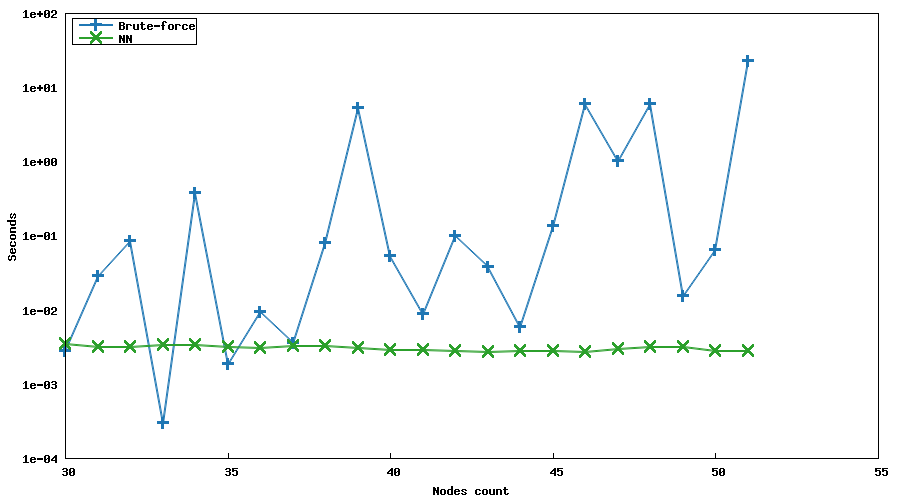
The blue graph doesn't behave like a nearly continuous function, but that's because sometimes the brute-force algorithm could get lucky and return the answer pretty soon. Most importantly, we can observe the trend. Also, generated with gnuplot.

Follow-up

After some more experimentation, it turned out it was possible to add some data augmentation. The biggest advantage is that there's going to be less room for overfitting. In other words, the model should not merely memorize the answer for specific graphs; instead, it should learn the topological nature of the longest path. I've tried embedding Gaussian noise, which is quite common for what I'm trying to achieve. However, a technique that makes more sense for graphs is not exactly that; it's dropping edges with a defined probability. In some sense, it is noise as well, because we confuse the model: for example, we might remove an edge critical for the path designated as the longest. However, that's really the goal — making it analyze the underlying structure of this path without focusing on unreliable details. To use more professional terminology, we aim for generalization.

Here's how I add it:

class Network(torch.nn.Module):
    def __init__(self, hidden_channels):
        super(Network, self).__init__()

        self.edge_dropout_p = 0.05

        ...

    def forward(self, x, edge_index, batch):
        h = GELU()(self.input_proj(x))
        h = self.proj_norm(h, batch)

        edges = edge_index
        edges, _ = dropout_edge(
            edge_index, 
            p=self.edge_dropout_p,
            force_undirected=True,
            training=self.training
        )
        
        ...

Does this modification offer a substantial improvement though? Well, let's run training on a triplet of seeds with and without the change. Measuring the peak validation loss across the three seeds leads me to these results:
With: avg 0.8178
Without: avg ~0.8105

That's only 5%, so it makes sense the difference is negligible. However, it's best to keep it for a certain level of data expansion, considering that we have only about 800 graphs. Duing inference, the accuracy on complicated graphs stays visually similar. For example: Graph #013 | True Path: 50.0 | Predicted: 48.0439

Closing notes

Successful approximations from this network indicate that, in reality, when an NP-hard problem needs to be solved, we must resort to heuristics. Is this going to result in an exact solution? Definitely not. But is this approach going to suffice in practice? Well, that seems very likely.

All Articles

• Longest path problem w/ heuristicsby Cyril Ulyanov01-09-2026
• Size does matter, actuallyby Nick Borș27-06-2026
• The most crucial accomplishment of Lev Landauby Cyril Ulyanov04-06-2026
• How geometry blends with calculusby Cyril Ulyanov22-04-2026
• Matrixby Anthony Slab18-02-2026
• Hiatusby Anthony Slab21-11-2025